Data User’s Guide (R)

Getting Started

This data user’s guide relies on the combined, upcoded 2019-2023 dataset. In the code chunk below, the raw data are labeled using a convenience function, factorize_df, from the open-source R package travelSurveyTools (link here). The function takes as input the value labels from the combined 2019-2023 codebook. See section Dataset Preparation, Quality Assurance, and Quality Control for more information.

Like the remainder of this Synthesis report, this user’s guide also includes data for only weighted households, to exclude those households that did not meet the criteria for weighting during the 2019-2021 re-weighting process, and also those 2023 outreach households that did not meet initial completion criteria for weighting (See Expansion and Weighting for more information).

To filter unweighted households from all tables in the Travel Behavior Inventory dataset, users can run the following commands in R:

weighted_hhs <- tbi$hh[!is.na(hh_weight) & hh_weight > 0, hh_id]

tbi <-
  lapply(
    tbi,
    function(dt) {
      dt <- dt[hh_id %in% weighted_hhs]
    }
  )

The resulting dataset, tbi, is a list of six tables in data.table format.

nrows <- lapply(tbi, nrow) %>%
  stack(.) %>%
  rename(., "Rows" = "values") %>%
  rename(., "Table" = "ind")

nrows %>%
  select(Table, Rows) %>%
  gt() %>%
  gt::fmt_number(columns = c(2), decimals = 0)

Table	Rows
hh	19,172
person	38,693
day	157,961
trip	623,926
vehicle	30,240
trip_purpose	844,728
linked_trip	609,725
hh_day	80,192

Basic Operations

Summarizing SRCVs: Single Response Categorical Variables

A single-response categorical variable (SRCV) is a column in the dataset containing answers for a question for which the survey respondent could select only one option from a list of pre-populated answers. For this example, use income_broad.

tbl <- tbi$hh %>%
  count(income_broad) %>%
  mutate(Percent = n / sum(n) * 100)

tbl %>%
  gt()

income_broad	n	Percent
Under $25,000	2480	12.935531
$25,000-$49,999	3169	16.529314
$50,000-$74,999	3279	17.103067
$75,000-$99,999	2816	14.688087
$100,000 or more	5861	30.570624
Prefer not to answer	1567	8.173378

tbl %>%
  ggplot(aes(x = as.factor(income_broad), y = Percent)) +
  geom_col(fill = councilR::colors$councilBlue) +
  labs(x = "Percent of Households", y = "Income, Broad Categories") +
  coord_flip() +
  councilR::theme_council()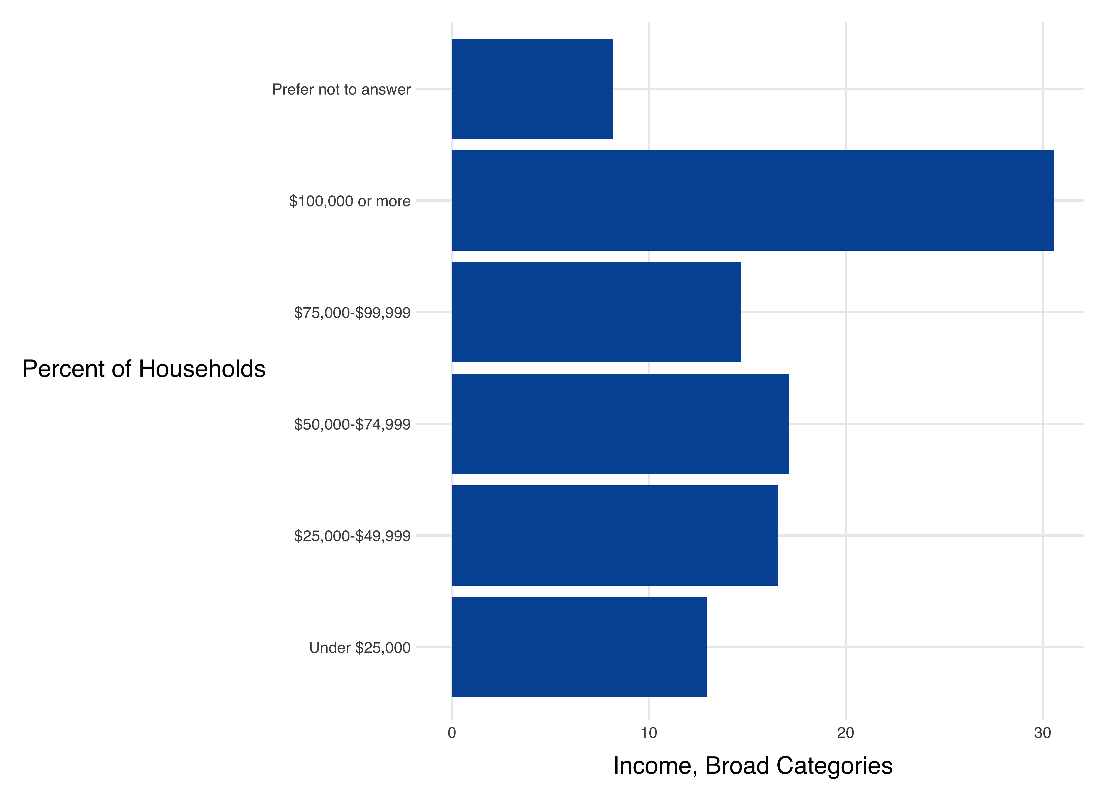

Be careful with count variables! Can’t simply take the mean:

tbi$hh %>%
  group_by(survey_year) %>%
  count(num_bicycles) %>%
  ungroup() %>%
  pivot_wider(names_from = survey_year, values_from = n) %>%
  gt::gt() %>%
  gt::sub_missing(columns = c(2:4))

num_bicycles	2019	2021	2023
NA	7516	—	—
0 (No bicycles)	—	2468	1217
1 bicycle	—	1944	893
2 bicycles	—	1693	775
3 bicycles	—	657	344
4 bicycles	—	522	258
5 bicycles	—	275	121
6 bicycles	—	126	65
7 bicycles	—	58	16
8 or more	—	101	44
Missing	—	63	16

Summarizing MRCVs: Multiple Response Categorical Variables

Some questions in the survey allow respondents to check multiple options. Common examples include questions about race and ethnicity, or reasons for not traveling. These checkbox variables, also known as multiple response categorical variables (MRCVs), are represented differently in the dataset from SRCVs (Single Response Categorical Variables) and have to be handled differently.

Let’s use no_travel as an example.

MRCV Names and Descriptions

What does the data actually look like for this question?

tbi$day %>%
  select(person_id, day_id, starts_with("no_travel")) %>%
  tail() %>%
  gt::gt()

person_id	day_id	no_travel_other_specify	no_travel_8	no_travel_9	no_travel_4	no_travel_5	no_travel_6	no_travel_2	no_travel_99	no_travel_7	no_travel_3	no_travel_11	no_travel_1	no_travel_12
2314127201	231412720103	NA	Missing	Missing	Missing	Missing	Missing	Missing	Missing	Missing	Missing	Missing	Missing	Missing
2311924101	231192410104	NA	Not selected	Not selected	Not selected	Not selected	Not selected	Not selected	Selected	Not selected	Not selected	Not selected	Not selected	Not selected
2302769301	230276930104	NA	Not selected	Not selected	Not selected	Not selected	Not selected	Selected	Not selected	Not selected	Not selected	Not selected	Not selected	Not selected
2303498001	230349800104	NA	Not selected	Not selected	Selected	Not selected	Not selected	Not selected	Not selected	Not selected	Not selected	Not selected	Not selected	Not selected
2312417001	231241700104	NA	Not selected	Not selected	Selected	Not selected	Not selected	Not selected	Not selected	Not selected	Not selected	Not selected	Not selected	Not selected
2315044102	231504410205	NA	Not selected	Not selected	Selected	Not selected	Not selected	Not selected	Not selected	Not selected	Not selected	Not selected	Not selected	Not selected

tbi$day %>%
  left_join(tbi$hh) %>%
  group_by(survey_year) %>%
  count(no_travel_11) %>%
  ungroup() %>%
  gt::gt()

Joining with `by = join_by(hh_id)`

survey_year	no_travel_11	n
2019	Not selected	6387
2019	Selected	889
2019	Missing	72280
2021	Not selected	7924
2021	Selected	458
2021	Missing	41185
2023	Not selected	4236
2023	Selected	355
2023	Missing	24247

Get the labels for these columns

nt_desc <- filter(variable_list, str_detect(variable, "no_travel")) %>%
  select(variable, description)

nt_desc %>%
  gt::gt()

variable	description
no_travel_1	Reason for no travel on date: I did make trips on date
no_travel_11	Reason for no travel on date: Weather conditions (e.g., snowstorm)
no_travel_12	Reason for no travel on date: person may have made trips, but I don't know when or where
no_travel_2	Reason for no travel on date: Not scheduled to work/took day off
no_travel_3	Reason for no travel on date: Worked at home for pay (e.g., telework, self-employed)
no_travel_4	Reason for no travel on date: Hung out around home
no_travel_5	Reason for no travel on date: Scheduled school closure (e.g., holiday)
no_travel_6	Reason for no travel on date: No available transportation (e.g., no car, no bus)
no_travel_7	Reason for no travel on date: Sick or quarantining (self or others)
no_travel_8	Reason for no travel on date: Waited for visitor/delivery (e.g., plumber)
no_travel_9	Reason for no travel on date: person did online/remote/home school
no_travel_99	Reason for no travel on date: Other reason
no_travel_other_specify	Other reason for no travel on date open text answer

Clean up labels by removing the common part.

nt_desc2 <- nt_desc %>%
  mutate(description = str_replace(
    description,
    "Reason for no travel on date: ",
    ""
  ))

nt_desc2 %>%
  gt::gt()

variable	description
no_travel_1	I did make trips on date
no_travel_11	Weather conditions (e.g., snowstorm)
no_travel_12	person may have made trips, but I don't know when or where
no_travel_2	Not scheduled to work/took day off
no_travel_3	Worked at home for pay (e.g., telework, self-employed)
no_travel_4	Hung out around home
no_travel_5	Scheduled school closure (e.g., holiday)
no_travel_6	No available transportation (e.g., no car, no bus)
no_travel_7	Sick or quarantining (self or others)
no_travel_8	Waited for visitor/delivery (e.g., plumber)
no_travel_9	person did online/remote/home school
no_travel_99	Other reason
no_travel_other_specify	Other reason for no travel on date open text answer

Remove parentheticals at the end.

nt_desc3 <- nt_desc2 %>%
  mutate(description = str_replace(
    description,
    " \\(.*\\)$",
    ""
  ))

nt_desc3 %>%
  gt::gt()

variable	description
no_travel_1	I did make trips on date
no_travel_11	Weather conditions
no_travel_12	person may have made trips, but I don't know when or where
no_travel_2	Not scheduled to work/took day off
no_travel_3	Worked at home for pay
no_travel_4	Hung out around home
no_travel_5	Scheduled school closure
no_travel_6	No available transportation
no_travel_7	Sick or quarantining
no_travel_8	Waited for visitor/delivery
no_travel_9	person did online/remote/home school
no_travel_99	Other reason
no_travel_other_specify	Other reason for no travel on date open text answer

Summarize MRCV Data

To summarize the data follow these steps:

• Select the columns
• Filter out all the days that are missing responses (i.e., they did travel)
• Filter out all the days that aren’t weighted (e.g. day not complete)
• Pivot data so we don’t have to work across columns
• Calculate the fraction of respondents that checked each option
• Label responses

Select the columns:

missing_value <- "Missing"

# Select the columns
nt_summary <-
  tbi$day %>%
  left_join(tbi$hh) %>%
  # select all the columns:
  select(survey_year, person_id, day_id, day_weight, starts_with("no_travel")) %>%
  # Get rid of open-ended text answer:
  select(-contains("other_specify"))

Joining with `by = join_by(hh_id)`

nt_summary %>%
  head(10) %>%
  gt()

survey_year	person_id	day_id	day_weight	no_travel_8	no_travel_9	no_travel_4	no_travel_5	no_travel_6	no_travel_2	no_travel_99	no_travel_7	no_travel_3	no_travel_11	no_travel_1	no_travel_12
2019	1822516701	182251670101	0	Missing	Missing	Missing	Missing	Missing	Missing	Missing	Missing	Missing	Missing	NA	NA
2019	1830175901	183017590101	0	Missing	Missing	Missing	Missing	Missing	Missing	Missing	Missing	Missing	Missing	NA	NA
2019	1831965201	183196520101	0	Missing	Missing	Missing	Missing	Missing	Missing	Missing	Missing	Missing	Missing	NA	NA
2019	1834127101	183412710101	0	Missing	Missing	Missing	Missing	Missing	Missing	Missing	Missing	Missing	Missing	NA	NA
2019	1834438301	183443830101	0	Missing	Missing	Missing	Missing	Missing	Missing	Missing	Missing	Missing	Missing	NA	NA
2019	1835758001	183575800101	0	Missing	Missing	Missing	Missing	Missing	Missing	Missing	Missing	Missing	Missing	NA	NA
2019	1836448001	183644800101	0	Missing	Missing	Missing	Missing	Missing	Missing	Missing	Missing	Missing	Missing	NA	NA
2019	1846241501	184624150101	0	Missing	Missing	Missing	Missing	Missing	Missing	Missing	Missing	Missing	Missing	NA	NA
2019	1849549501	184954950101	0	Missing	Missing	Missing	Missing	Missing	Missing	Missing	Missing	Missing	Missing	NA	NA
2019	1850835001	185083500101	0	Missing	Missing	Missing	Missing	Missing	Missing	Missing	Missing	Missing	Missing	NA	NA

Filter and pivot the data:

nt_summary <-
  nt_summary %>%
  # Filter out all the rows that aren't weighted (e.g. day not complete)
  filter(
    !is.na(day_weight) & day_weight > 0
  ) %>%
  filter(
    !if_all(starts_with("no_travel"), ~ . %in% c("Missing", NA))
  ) %>%
  pivot_longer(cols = starts_with("no_travel"), names_to = "variable")


nt_summary %>%
  head(10) %>%
  gt()

survey_year	person_id	day_id	day_weight	variable	value
2019	1981190301	198119030102	29.49463	no_travel_8	Not selected
2019	1981190301	198119030102	29.49463	no_travel_9	Not selected
2019	1981190301	198119030102	29.49463	no_travel_4	Selected
2019	1981190301	198119030102	29.49463	no_travel_5	Not selected
2019	1981190301	198119030102	29.49463	no_travel_6	Not selected
2019	1981190301	198119030102	29.49463	no_travel_2	Not selected
2019	1981190301	198119030102	29.49463	no_travel_99	Not selected
2019	1981190301	198119030102	29.49463	no_travel_7	Not selected
2019	1981190301	198119030102	29.49463	no_travel_3	Not selected
2019	1981190301	198119030102	29.49463	no_travel_11	Not selected

Calculate the fraction of respondents that checked each option:

nt_summary <-
  nt_summary %>%
  # Remove missing responses
  filter(value != "Missing") %>%
  filter(!is.na(value)) %>%
  group_by(survey_year, variable, value) %>%
  summarize(
    wtd_num = sum(day_weight)
  ) %>%
  ungroup() %>%
  group_by(survey_year, variable) %>%
  mutate(wtd_pct = wtd_num / sum(wtd_num)) %>%
  ungroup()

`summarise()` has grouped output by 'survey_year', 'variable'. You can override
using the `.groups` argument.

nt_summary %>%
  head(10) %>%
  gt()

survey_year	variable	value	wtd_num	wtd_pct
2019	no_travel_1	NA	461644.29	1.0000000
2019	no_travel_11	Not selected	379270.90	0.8215652
2019	no_travel_11	Selected	82373.39	0.1784348
2019	no_travel_12	NA	461644.29	1.0000000
2019	no_travel_2	Not selected	182081.96	0.8066498
2019	no_travel_2	Selected	43644.20	0.1933502
2019	no_travel_3	Not selected	185662.81	0.8225135
2019	no_travel_3	Selected	40063.35	0.1774865
2019	no_travel_4	Not selected	295412.61	0.6399139
2019	no_travel_4	Selected	166231.68	0.3600861

Label responses and format table:

# Label responses
nt_summary <-
  nt_summary %>%
  # Label Responses
  left_join(nt_desc3, by = "variable")

# Put survey year in separate columns, format;
nt_summary %>%
  # Filter to the percent that "Selected" the response option:
  filter(value == "Selected") %>%
  filter(!is.na(value)) %>%
  select(survey_year, variable, description, wtd_pct) %>%
  pivot_wider(names_from = "survey_year", values_from = "wtd_pct") %>%
  gt() %>%
  gt::fmt_percent(columns = c(3:5), decimals = 1) %>%
  gt::sub_missing(columns = c(3:5), missing_text = "--")

variable	description	2019	2021	2023
no_travel_11	Weather conditions	17.8%	4.1%	8.9%
no_travel_2	Not scheduled to work/took day off	19.3%	12.5%	10.9%
no_travel_3	Worked at home for pay	17.7%	22.0%	22.3%
no_travel_4	Hung out around home	36.0%	52.3%	47.0%
no_travel_5	Scheduled school closure	7.7%	1.6%	2.8%
no_travel_6	No available transportation	2.6%	1.2%	1.5%
no_travel_7	Sick or quarantining	12.0%	6.2%	6.3%
no_travel_8	Waited for visitor/delivery	1.4%	1.6%	1.1%
no_travel_9	person did online/remote/home school	0.9%	2.8%	3.2%
no_travel_99	Other reason	14.1%	11.3%	11.4%
no_travel_1	I did make trips on date	–	1.0%	1.1%
no_travel_12	person may have made trips, but I don't know when or where	–	0.7%	1.2%

Working with Weights

Weighted proportions are calculated here in two different ways. First, they are calculated manually to illustrate a simple approach.

Second, the {srvyr} package (basically a wrapper around the {survey} package) is demonstrated to calculate standard errors and confidence intervals as well as the proportions themselves.

Weighted Proportions

To calculate weighted proportions, or weighted counts, we simply sum the weights instead of counting the number of rows.

tbl <- tbi$hh %>%
  group_by(income_broad) %>%
  summarize(N = n(), wtd_N = sum(hh_weight)) %>%
  mutate(prop = N / sum(N), wtd_prop = wtd_N / sum(wtd_N)) %>%
  ungroup()

tbl %>%
  gt::gt() %>%
  gt::fmt_number(columns = c(2:3), decimals = 0) %>%
  gt::fmt_percent(columns = c(4:5), decimals = 1)

income_broad	N	wtd_N	prop	wtd_prop
Under $25,000	2,480	620,099	12.9%	13.7%
$25,000-$49,999	3,169	813,693	16.5%	18.0%
$50,000-$74,999	3,279	644,296	17.1%	14.3%
$75,000-$99,999	2,816	567,726	14.7%	12.6%
$100,000 or more	5,861	1,501,144	30.6%	33.2%
Prefer not to answer	1,567	372,129	8.2%	8.2%

tbl %>%
  ggplot(aes(x = income_broad, y = wtd_prop)) +
  geom_col(fill = councilR::colors$councilBlue) +
  councilR::theme_council_open() +
  coord_flip()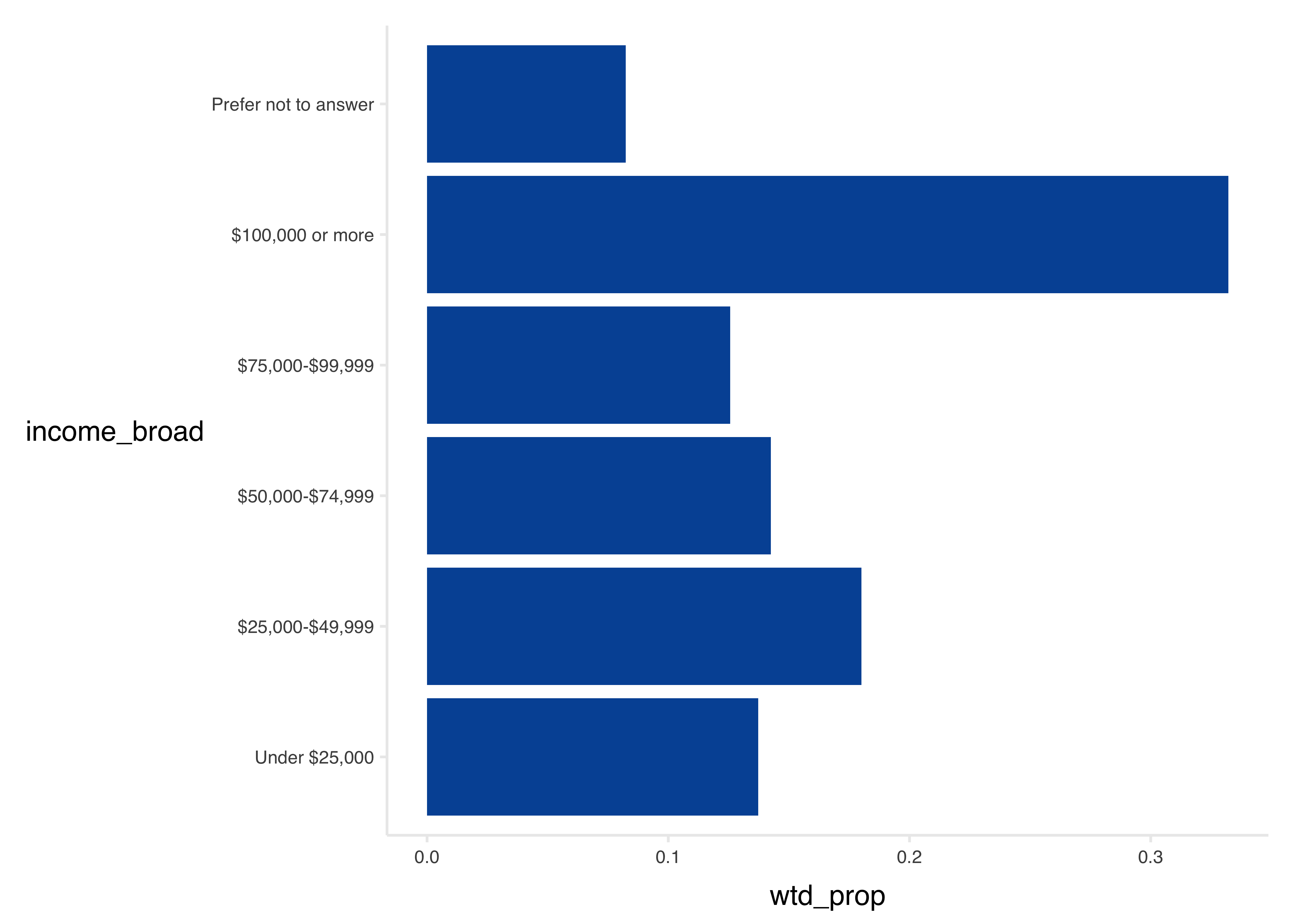

Using the {srvyr} Package

Here the {srvyr} package is used to calculate the standard error as well.

The {srvyr} package uses a design object instead of the data directly. This contains information about the survey design.

# Define the design
hh_design <- tbi$hh %>%
  filter(!is.na(hh_weight)) %>%
  as_survey_design(
    ids = hh_id,
    weights = hh_weight,
    strata = sample_segment
  )

tbl <- hh_design %>%
  group_by(income_broad) %>%
  summarize(
    N = n(),
    wtd_est = survey_total(vartype = "se"),
    wtd_prop = survey_prop(vartype = "se", proportion = TRUE)
  ) %>%
  ungroup()


tbl %>%
  gt::gt() %>%
  gt::fmt_number(columns = c(2:4), decimals = 0) %>%
  gt::fmt_percent(columns = c(5:6), decimals = 1)

income_broad	N	wtd_est	wtd_est_se	wtd_prop	wtd_prop_se
Under $25,000	2,480	620,099	20,079	13.7%	0.4%
$25,000-$49,999	3,169	813,693	22,047	18.0%	0.5%
$50,000-$74,999	3,279	644,296	19,284	14.3%	0.4%
$75,000-$99,999	2,816	567,726	18,379	12.6%	0.4%
$100,000 or more	5,861	1,501,144	31,250	33.2%	0.6%
Prefer not to answer	1,567	372,129	15,522	8.2%	0.3%

tbl %>%
  ggplot(aes(x = income_broad, y = wtd_prop)) +
  geom_col(fill = councilR::colors$councilBlue) +
  geom_linerange(
    aes(ymin = wtd_prop - wtd_prop_se, ymax = wtd_prop + wtd_prop_se)
  ) +
  coord_flip() +
  councilR::theme_council_open()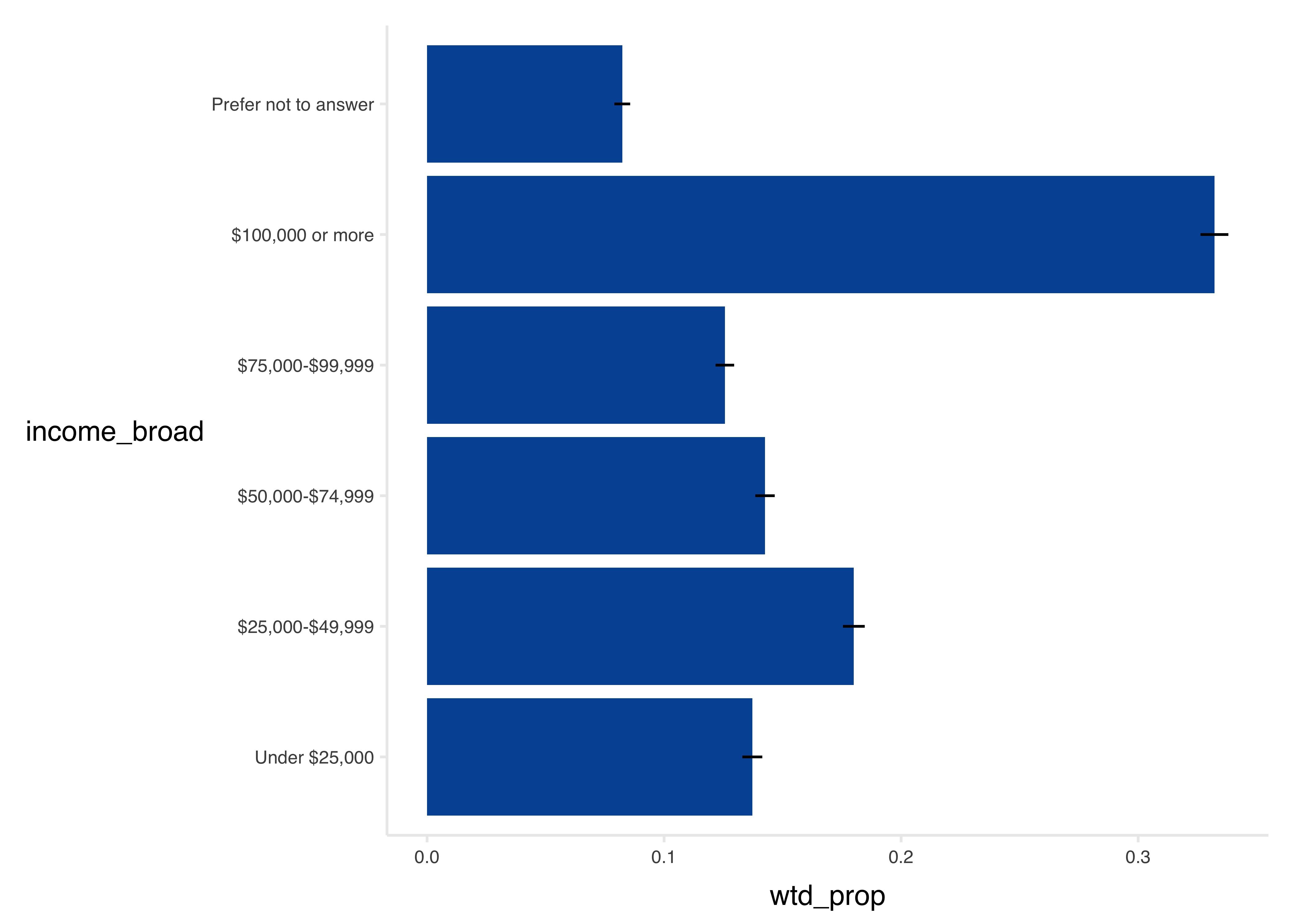

A Note on Sample Strata

In the code above, the survey design specifies strata, corresponding to the sample segments from the sample plan. Specifying strata improves the precision of confidence intervals and standard errors, but does not change the point estimates.

In survey data analysis, strata are used to ensure that the sample is representative of key subgroups in the population or when survey sampling rates differed across subpopulations or subgeographies. In the Travel Behavior Inventory, Core Urban sample segments were oversampled, and hence strata specification (using sample segments as strata) is warranted.

Failing to specify strata, while not exactly correct, rarely has more than a miniscule effect on error estimates. In the example below, we show how confidence intervals are affected by specifying strata in the survey design object.

Weighted Proportion by Another Variable

Calculating proportions grouped by another variable requires some thought as to the weights applied.

Variables in the Same Table

Here we calculate income by home county. Both variables are household-level variables, so household weights are applied.

tbl %>%
  mutate(home_county = gsub(" County, MN| County, WI", "", home_county)) %>%
  ggplot(aes(x = income_broad, y = wtd_prop)) +
  geom_col(fill = councilR::colors$councilBlue) +
  geom_linerange(
    aes(ymin = wtd_prop - wtd_prop_se, ymax = wtd_prop + wtd_prop_se)
  ) +
  coord_flip() +
  facet_wrap(~home_county) +
  councilR::theme_council_open()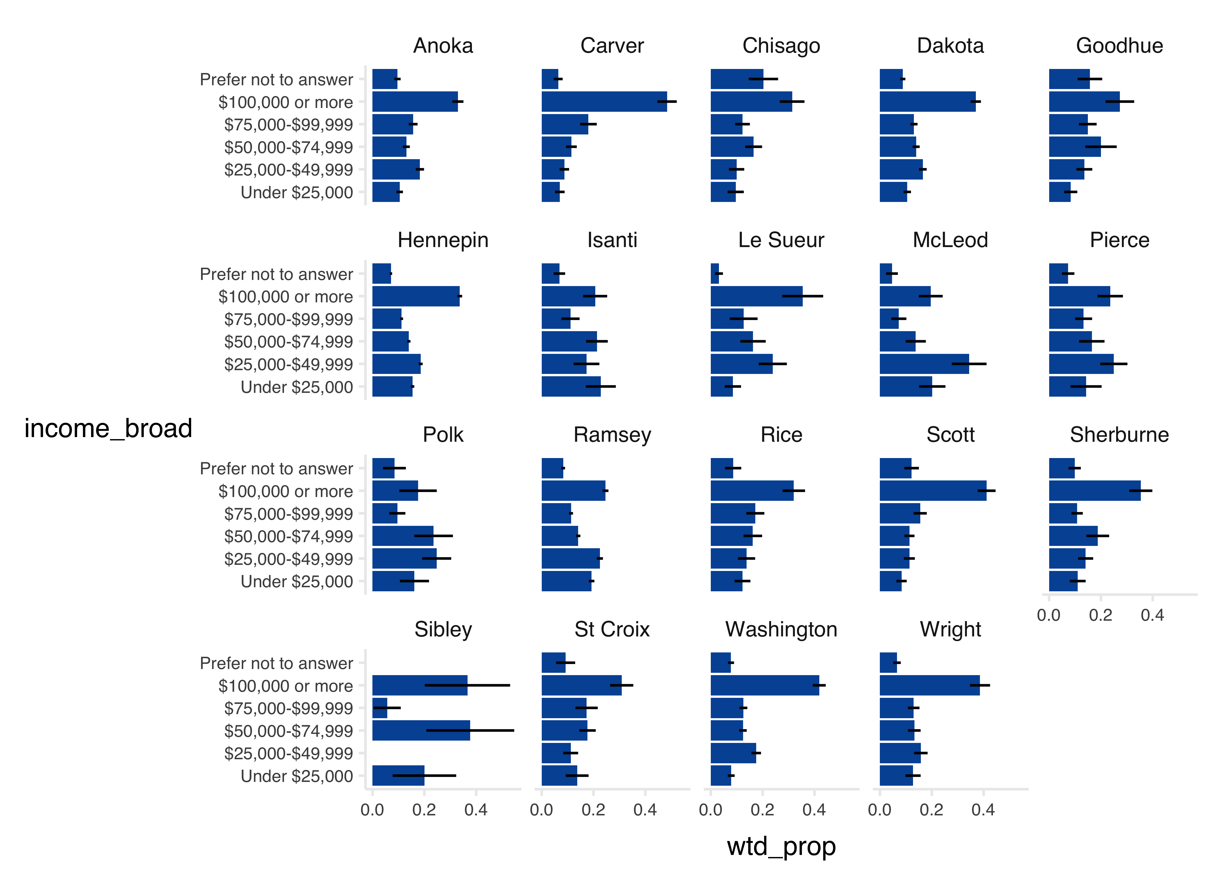

Variables in Different Tables

When the crosstab variables are in different tables, the general rule of thumb is to use the weight from the lowest level of the weighting hierarchy: trip weights, day weights, person weights, and finally household weights.

Weight to Use When Creating Weighted Crosstabs for Variables From One or Two Tables
		TABLE 2
		hh	vehicle	person	day	trip	trip_purpose
TABLE 1	hh	hh_weight
	vehicle	hh_weight	hh_weight
	person	person_weight	person_weight	person_weight
	day	day_weight	day_weight	day_weight	day_weight
	trip	trip_weight	trip_weight	trip_weight	trip_weight	trip_weight
	trip_purpose*	trip_purpose_weight	trip_purpose_weight	trip_purpose_weight	trip_purpose_weight	**	trip_purpose_weight
*This table is provided solely for analyses of overall trip purpose. **Do not join without first aggregating trip measures to linked trip IDs.

Example 1: Telework by County

For example, to find the proportion of people who teleworked part-time before the pandemic (a person-level variable) by home county (a household-level variable), the data user joins the household and person tables, then summarizes the person weight for a weighted estimate.

tab <- tbi$person %>%
  left_join(tbi$hh, by = "hh_id") %>%
  filter(survey_year == 2023) %>%
  group_by(home_county, job_type_pre_covid) %>%
  summarize(wtd_population = sum(person_weight)) %>%
  ungroup() %>%
  group_by(home_county) %>%
  mutate(wtd_prop_population = wtd_population / sum(wtd_population)) %>%
  ungroup()

`summarise()` has grouped output by 'home_county'. You can override using the
`.groups` argument.

tab %>%
  head(12) %>%
  gt::gt() %>%
  gt::fmt_percent(columns = 4) %>%
  gt::fmt_number(columns = 3, decimals = 0)

home_county	job_type_pre_covid	wtd_population	wtd_prop_population
Anoka County, MN	Went to one work location ONLY (outside of home)	142,719	42.30%
Anoka County, MN	Work location regularly varied (different offices/jobsites)	10,191	3.02%
Anoka County, MN	Worked ONLY from home or remotely (telework, self-employed)	10,790	3.20%
Anoka County, MN	Drove/biked/traveled for work (driver, sales, deliveries)	2,366	0.70%
Anoka County, MN	Teleworked some days and traveled to a work location some days	10,012	2.97%
Anoka County, MN	Missing	161,314	47.81%
Carver County, MN	Went to one work location ONLY (outside of home)	39,615	35.90%
Carver County, MN	Work location regularly varied (different offices/jobsites)	4,480	4.06%
Carver County, MN	Worked ONLY from home or remotely (telework, self-employed)	6,967	6.31%
Carver County, MN	Teleworked some days and traveled to a work location some days	5,048	4.58%
Carver County, MN	Missing	54,226	49.15%
Chisago County, MN	Went to one work location ONLY (outside of home)	26,314	53.18%

Example 2: Trip Distance by Mode

In this second example, we find the percent of trips that are under 1, 5, or 10 miles for each mode. This kind of analysis might be used to answer the question what percent of drive trips are short enough that they might be shifted to [walking/biking]? In this example, we use srvyr to get both the weighted proportions and their standard errors.

The results below show that, in 2023, 15.6% of drive drips were less than 1 mile long, compared to 84.5% of walk trips.

tab <- tbi$trip %>%
  left_join(select(tbi$hh, "hh_id", "sample_segment", "survey_year")) %>%
  filter(!is.na(distance_miles)) %>%
  filter(survey_year == 2023) %>%
  mutate(distance_category = case_when(distance_miles < 1 ~ "Less than 1 mile",
    distance_miles < 5 ~ "1-5 miles",
    distance_miles < 10 ~ "5-10 miles",
    distance_miles >= 10 ~ "10 miles or more",
    .default = "Missing"
  )) %>%
  as_survey_design(
    ids = trip_id,
    weights = trip_weight,
    strata = sample_segment
  ) %>%
  group_by(survey_year, mode_type, distance_category) %>%
  summarize(prop = survey_prop(proportion = FALSE)) %>%
  ungroup()

Joining with `by = join_by(hh_id)`

tab %>%
  mutate(distance_category = factor(distance_category,
    levels = c(
      "Less than 1 mile",
      "1-5 miles",
      "5-10 miles",
      "10 miles or more"
    )
  )) %>%
  arrange(mode_type, distance_category) %>%
  filter(mode_type %in% c("Walk", "Household Vehicle")) %>%
  head(12) %>%
  gt::gt() %>%
  gt::fmt_percent(columns = 4:5, decimals = 1)

survey_year	mode_type	distance_category	prop	prop_se
2023	Household Vehicle	Less than 1 mile	15.6%	0.4%
2023	Household Vehicle	1-5 miles	43.0%	0.5%
2023	Household Vehicle	5-10 miles	18.7%	0.4%
2023	Household Vehicle	10 miles or more	22.7%	0.5%
2023	Walk	Less than 1 mile	84.5%	1.0%
2023	Walk	1-5 miles	12.6%	0.9%
2023	Walk	5-10 miles	1.3%	0.4%
2023	Walk	10 miles or more	1.5%	0.4%

Sample Analyses

Weighted Trip Rates

To calculate a weighted trip rate (the number of trips per day), the number of weighted trips is divided by the number of weighted travel days.

For example:

• If there are 300,000 weighted person-trips across 75,000 person-days, then the average person-trip rate is 4.0 per day.
• If there are 225,000 person-trips by car across 75,000 person-days, then the person-trip rate for car trips is 3.0.

Note: Travel days with no trips are not represented in the trip table! They must be obtained by performing a join on the day table.

Weighted trip rates can either be calculated using the unlinked trip table (trip), or the linked trip table (linked_trip). The unlinked trip rate represents the number of trips made inclusive of multi-part journeys, like walking to a bus stop. The linked trip table consolidates these multi-trip journeys into a single trip record. As a result, linked trip rates are always lower than unlinked trip rates.

trip_counts <- tbi$trip %>%
  filter(!is.na(trip_weight) & trip_weight > 0) %>%
  group_by(day_id) %>%
  summarize(wtd_num_trips = sum(trip_weight)) %>%
  ungroup()

trip_counts %>%
  tail(10) %>%
  gt::gt()

day_id	wtd_num_trips
231735820302	1439.4171
231735820402	1439.4171
231735820502	1439.4171
231737120101	1335.3016
231737120201	1573.3379
231737120301	511.6536
231737120401	255.8268
231737990101	989.7791
231737990102	395.9116
231737990103	791.8233

# Join to day table

trip_counts <- tbi$day %>%
  filter(day_weight > 0) %>%
  select(hh_id, day_id, day_weight) %>%
  left_join(trip_counts, by = "day_id") %>%
  left_join(select(tbi$hh, hh_id, sample_segment, income_broad), by = "hh_id")


trip_counts %>%
  tail(10) %>%
  gt::gt()

hh_id	day_id	day_weight	wtd_num_trips	sample_segment	income_broad
23034980	230349800107	62.45773	NA	Core Urban BGs	$100,000 or more
23050326	230503260101	734.23731	NA	Core Urban BGs	Prefer not to answer
23088895	230888950101	50.31765	123.4231	Core Urban BGs	$50,000-$74,999
23049602	230496020301	2573.17431	NA	Core Urban BGs	$100,000 or more
23033885	230338850301	512.73826	1061.1328	Core Urban BGs	$100,000 or more
23150441	231504410202	115.50532	NA	Core Rural	$75,000-$99,999
23125965	231259650203	99.00411	198.0082	Core Urban BGs	$100,000 or more
23003220	230032200103	34.53968	NA	Core Urban BGs	Under $25,000
23092788	230927880205	99.07492	693.5245	Core Urban BGs	$100,000 or more
23089592	230895920105	49.98151	NA	Core Urban BGs	$100,000 or more

Replace the NAs with 0s.

trip_counts <- trip_counts %>%
  mutate(wtd_num_trips = replace_na(wtd_num_trips, 0))

trip_counts %>%
  tail(10) %>%
  gt::gt()

hh_id	day_id	day_weight	wtd_num_trips	sample_segment	income_broad
23034980	230349800107	62.45773	0.0000	Core Urban BGs	$100,000 or more
23050326	230503260101	734.23731	0.0000	Core Urban BGs	Prefer not to answer
23088895	230888950101	50.31765	123.4231	Core Urban BGs	$50,000-$74,999
23049602	230496020301	2573.17431	0.0000	Core Urban BGs	$100,000 or more
23033885	230338850301	512.73826	1061.1328	Core Urban BGs	$100,000 or more
23150441	231504410202	115.50532	0.0000	Core Rural	$75,000-$99,999
23125965	231259650203	99.00411	198.0082	Core Urban BGs	$100,000 or more
23003220	230032200103	34.53968	0.0000	Core Urban BGs	Under $25,000
23092788	230927880205	99.07492	693.5245	Core Urban BGs	$100,000 or more
23089592	230895920105	49.98151	0.0000	Core Urban BGs	$100,000 or more

Finally, calculate the mean. Note that it is not appropriate to calculate the mean trip rate with the mean function.

trip_counts %>%
  summarize(
    N = n(),
    correct = sum(wtd_num_trips) / sum(day_weight),
    INCORRECT = mean(wtd_num_trips / day_weight)
  ) %>%
  gt::gt()

N	correct	INCORRECT
64015	3.544836	4.031447

As a simple demonstration of why there is a difference:

foo <- data.frame(trips = c(2, 10), days = c(2, 5))
foo %>%
  gt::gt()

trips	days
2	2
10	5

foo %>%
  summarize(
    correct = sum(trips) / sum(days),
    INCORRECT = mean(trips / days)
  ) %>%
  gt::gt() %>%
  gt::fmt_number(columns = c(1:2), decimals = 2)

correct	INCORRECT
1.71	1.50

To use srvyr, simply specify the calculation in the call to survey_mean.

tc_design <- trip_counts %>%
  as_survey_design(
    ids = day_id,
    weights = day_weight,
    strata = sample_segment
  )

tc_design %>%
  summarize(
    N = n(),
    wtd_trip_rate = survey_mean(wtd_num_trips / day_weight)
  ) %>%
  gt() %>%
  gt::fmt_number(columns = c(2:3), decimals = 2)

N	wtd_trip_rate	wtd_trip_rate_se
64015	3.54	0.02

Calculate by group as well.

tc_design %>%
  group_by(income_broad) %>%
  summarize(
    N = n(),
    wtd_trip_rate = survey_mean(wtd_num_trips / day_weight)
  ) %>%
  ungroup() %>%
  gt() %>%
  gt::fmt_number(columns = c(2), decimals = 0) %>%
  gt::fmt_number(columns = c(3:4), decimals = 2)

income_broad	N	wtd_trip_rate	wtd_trip_rate_se
Under $25,000	5,315	3.24	0.09
$25,000-$49,999	8,182	3.45	0.07
$50,000-$74,999	10,042	3.49	0.06
$75,000-$99,999	10,481	3.66	0.07
$100,000 or more	25,721	3.72	0.04
Prefer not to answer	4,274	3.09	0.08

To recap, when calculating a simple aggregate trip rate, joins are made to the day table to account for days without travel. The user:

• Gets the weighted number of trips for each day from the trip table.
• Joins to the day table.
• Fills in the weighted number of trips with zeros for those days without travel.

Summary statistics can then be created from the weighted number of trips divided by the day weight. The code below consolidates the example walk through from above:

trip_counts <- tbi$trip %>%
  filter(!is.na(trip_weight) & trip_weight > 0) %>%
  group_by(day_id) %>%
  summarize(wtd_num_trips = sum(trip_weight)) %>%
  ungroup()

trip_counts <- tbi$day %>%
  filter(day_weight > 0) %>%
  select(hh_id, day_id, day_weight) %>%
  left_join(trip_counts, by = "day_id") %>%
  left_join(select(tbi$hh, hh_id, sample_segment, survey_year),
    by = "hh_id"
  )

trip_counts <- trip_counts %>%
  mutate(wtd_num_trips = replace_na(wtd_num_trips, 0))

trip_counts %>%
  as_survey_design(
    ids = day_id,
    weights = day_weight,
    strata = sample_segment
  ) %>%
  group_by(survey_year) %>%
  summarize(
    N = n(),
    wtd_trip_rate = survey_mean(wtd_num_trips / day_weight)
  ) %>%
  ungroup() %>%
  gt() %>%
  gt::fmt_number(columns = c(2), decimals = 0) %>%
  gt::fmt_number(columns = c(3:4), decimals = 2)

survey_year	N	wtd_trip_rate	wtd_trip_rate_se
2019	32,150	4.19	0.04
2021	20,780	2.87	0.04
2023	11,085	3.58	0.05

Special Case: Trip Rates by a Trip Variable

When calculating trip rates by a trip attribute (i.e., a variable in the trip table) the user must not only account for days without travel, but also days without trips that match that attribute. In the case of mode type, this requires an expansion of the dataset to encompass every day, and every mode.

For example, to find trip rates by mode, the user:

• Calculates the weighted number of trips by mode and day ID.

• Expands the trip count data frame to include days without travel by each mode. In the code below, this is done by creating an empty data frame containing every combination of day_id and mode_type.

• Fills in missing values for the weighted number of trips with zeros, representing days without travel by that mode type.

# Weighted number of trips by mode type and day:
trip_counts <- tbi$trip %>%
  filter(!is.na(trip_weight) & trip_weight > 0) %>%
  group_by(day_id, mode_type) %>%
  summarize(wtd_num_trips = sum(trip_weight)) %>%
  ungroup()

`summarise()` has grouped output by 'day_id'. You can override using the
`.groups` argument.

# An empty data frame to hold every combination of day id and
empty_grid <- expand.grid(
  day_id = tbi$day$day_id,
  mode_type = levels(tbi$trip$mode_type)
)

empty_grid$mode_type <- factor(empty_grid$mode_type,
  levels = levels(tbi$trip$mode_type),
  ordered = TRUE
)

all_levels <- union(levels(trip_counts$mode_type), levels(empty_grid$mode_type))

# Align levels
trip_counts$mode_type <- factor(trip_counts$mode_type, levels = all_levels, ordered = TRUE)
empty_grid$mode_type <- factor(empty_grid$mode_type, levels = all_levels, ordered = TRUE)

# Join to our empty grid of modes and days:
trip_counts <- empty_grid %>%
  left_join(trip_counts, by = c("day_id", "mode_type")) # can you fill NAs with zeros here?

# Fill in zeros:
trip_counts <- trip_counts %>%
  mutate(wtd_num_trips = nafill(wtd_num_trips, fill = 0))

trip_counts %>%
  head(10) %>%
  gt()

day_id	mode_type	wtd_num_trips
182251670101	Rail	0
183017590101	Rail	0
183196520101	Rail	0
183412710101	Rail	0
183443830101	Rail	0
183575800101	Rail	0
183644800101	Rail	0
184624150101	Rail	0
184954950101	Rail	0
185083500101	Rail	0

Once created, the expanded table of trip counts can be joined to other, non-trip tables and summarized in the same manner as other trip rate crosstabs. For example, to calculate trip rate by home county and mode type:

trip_counts %>%
  left_join(tbi$day) %>%
  left_join(tbi$hh) %>%
  group_by(survey_year, home_county, mode_type) %>%
  summarize(trip_rate = sum(wtd_num_trips) / sum(day_weight)) %>%
  ungroup() %>%
  head(10) %>%
  gt()

Joining with `by = join_by(day_id)`
Joining with `by = join_by(hh_id)`
`summarise()` has grouped output by 'survey_year', 'home_county'. You can
override using the `.groups` argument.

survey_year	home_county	mode_type	trip_rate
2019	Anoka County, MN	Rail	0.003992510
2019	Anoka County, MN	School Bus	0.078010777
2019	Anoka County, MN	Public Bus	0.033112483
2019	Anoka County, MN	Other Bus	0.018334470
2019	Anoka County, MN	Long distance passenger mode	0.002931250
2019	Anoka County, MN	Smartphone ridehailing service	0.001922443
2019	Anoka County, MN	For-Hire Vehicle	0.001066327
2019	Anoka County, MN	Household Vehicle	3.434414204
2019	Anoka County, MN	Other Vehicle	0.180770027
2019	Anoka County, MN	Micromobility	0.023927973

To extend this process to multiple trip variables, such as trip mode and trip departure hour, the empty data frame simply needs to be expanded to include the second variable before joining and filling in days without travel.

empty_grid <- expand.grid(
  day_id = tbi$day$day_id,
  mode_type = value_labels_upcoded[variable == "mode_type", value],
  depart_hour = 0:23
)

empty_grid %>%
  head(10) %>%
  gt()

day_id	mode_type	depart_hour
182251670101	1	0
183017590101	1	0
183196520101	1	0
183412710101	1	0
183443830101	1	0
183575800101	1	0
183644800101	1	0
184624150101	1	0
184954950101	1	0
185083500101	1	0

Weighted Mode Share

Mode share represents the proportion of trips taken by walking, driving, biking, transit, and other modes. It is calculated from the linked trip table.

Prepare the design object for srvyr:

trips1 <- tbi$linked_trip %>%
  left_join(select(tbi$hh, hh_id, sample_segment), by = "hh_id") %>%
  filter(!is.na(linked_trip_weight) & linked_trip_weight > 0)

trip_design <- trips1 %>%
  as_survey_design(
    ids = linked_trip_id,
    weights = linked_trip_weight,
    strata = sample_segment
  )

Calculate and label:

tbl <- trip_design %>%
  group_by(mode_type) %>%
  summarize(
    N = n(),
    wtd_N = sum(linked_trip_weight),
    wtd_prop = survey_prop(vartype = "se", proportion = TRUE)
  ) %>%
  ungroup()

tbl %>%
  select(mode_type, N, wtd_N, wtd_prop, wtd_prop_se) %>%
  arrange(desc(wtd_prop)) %>%
  gt::gt() %>%
  gt::fmt_number(columns = c(2:3), decimals = 0) %>%
  gt::fmt_percent(columns = c(4:5), decimals = 1) %>%
  gt::sub_small_vals(threshold = 0.001, small_pattern = "<0.1%")

mode_type	N	wtd_N	wtd_prop	wtd_prop_se
Household Vehicle	180,512	31,374,063	80.3%	0.2%
Walk	29,051	3,437,077	8.8%	0.1%
Other Vehicle	13,277	1,913,337	4.9%	<0.1%
School Bus	2,876	716,939	1.8%	<0.1%
Micromobility	3,734	391,142	1.0%	<0.1%
Public Bus	4,596	376,769	1.0%	<0.1%
Other	1,856	286,898	0.7%	<0.1%
Smartphone ridehailing service	901	129,296	0.3%	<0.1%
Missing	476	118,171	0.3%	<0.1%
Other Bus	806	116,212	0.3%	<0.1%
Rail	1,841	91,470	0.2%	<0.1%
Long distance passenger mode	400	57,953	0.1%	<0.1%
For-Hire Vehicle	219	48,910	0.1%	<0.1%

Plot:

tbl <- tbl %>%
  mutate(mode_type = mode_type %>%
    fct_reorder(wtd_prop) %>%
    fct_relevel("Other"))

ggplot(tbl, aes(x = mode_type, y = wtd_prop)) +
  geom_col(fill = councilR::colors$councilBlue) +
  geom_linerange(
    aes(ymin = wtd_prop - wtd_prop_se, ymax = wtd_prop + wtd_prop_se),
    linewidth = 1.2
  ) +
  coord_flip() +
  labs(
    title = "Mode share of trips",
    x = "",
    y = "Weighted proportion"
  ) +
  councilR::theme_council_open()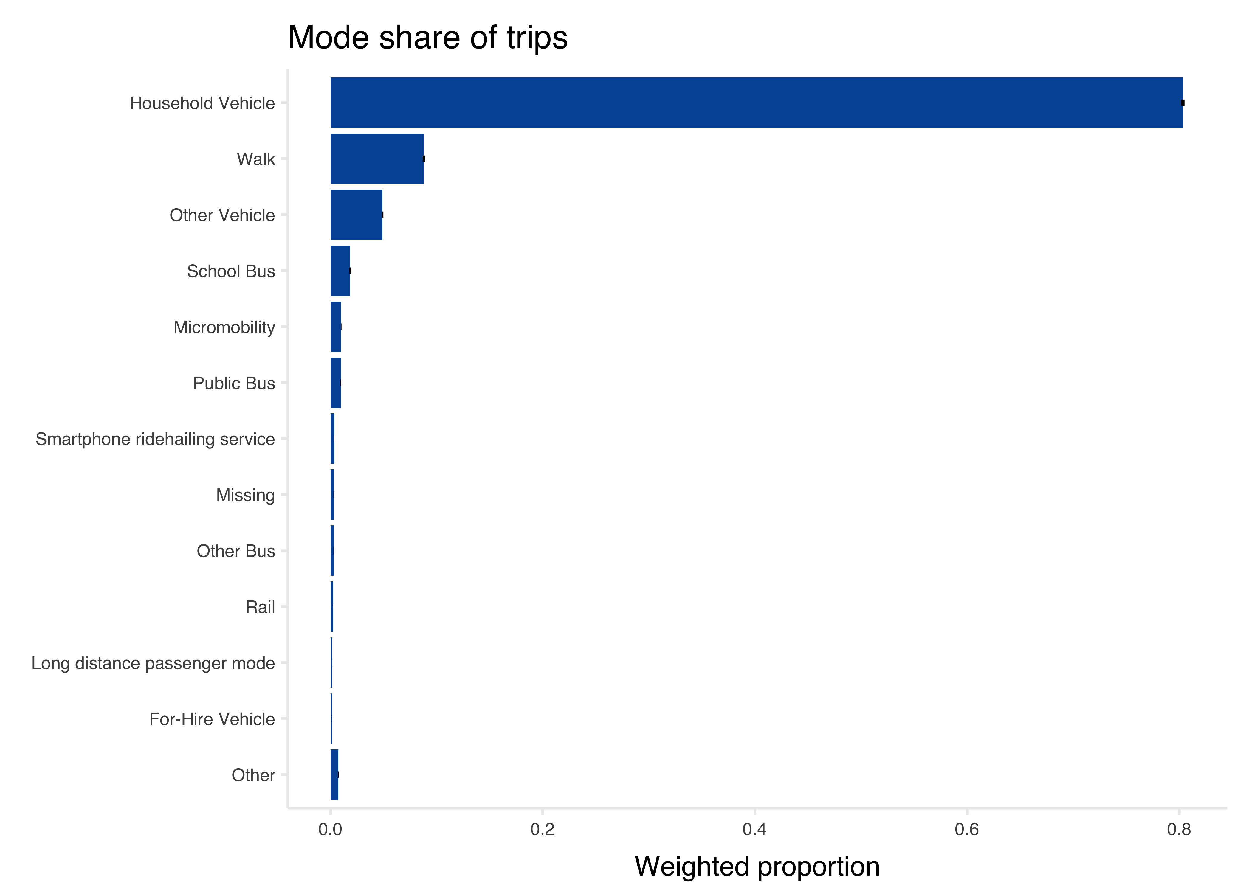

Weighted Purpose Share

Assigning the purpose to a trip can be done in a few ways. In previous analyses of the Travel Behavior Inventory data, trip purpose has been aggregated in one of two ways:

1. The user could use the destination place type (d_purpose, d_purpose_category)
   
2. The user can account for the origin and destination at the same time, by grouping trips into the tour type used during modeling (e.g., categorize trips as home-based work, home-based other, or non-home-based trips). This is typically the approach used in modeling.

RSG has provided a third option with the trip_purpose table. This table allows users to calculate aggregate, purpose-related statistics that accounts for the origin and destination place types of trips, in a manner more in keeping with the way a layperson might describe the purpose of their travel.

The trip_purpose table:

1. Re-links transit trips to minimize change mode purposes in the final trip purpose dataset. Some change mode purposes will still be present, for long-distance trips.
   
2. Divides linked trips into two categories: those with a home end, and those without.
   
3. For trips with a home end, the purpose of the trip is the destination place type of the non-home end. For example, a trip from home to work receives the purpose of work. The weight for the trip purpose record is equal to the original weight of the trip.
   
4. For trips without a home end, the purpose of the trip is shared equally between the origin end and destination end. For example, a trip from grocery shopping to school has the purpose of both shopping and school. The single trip is divided into two trip_purpose records, one for the grocery shopping end and a second for the school end. Half of the original trip weight is assigned to the grocery shop trip, with the other half to the school trip.

The end result is a table with fewer original trips than the trip table, owing to transit-trip re-linking; and more rows than the original trip table, owing to the creation of duplicate records for non-home-based trips.

Trip purpose by the destination place type

Note that home is the predominant purpose (destination place type).

tbl <-
  tbi$trip %>%
  left_join(tbi$hh) %>%
  filter(survey_year == 2023) %>%
  as_survey_design(
    weights = "trip_weight",
    ids = "trip_id",
    strata = "sample_segment"
  ) %>%
  group_by(d_purpose_category) %>%
  summarize(prop = survey_prop(proportion = TRUE, se = TRUE)) %>%
  ungroup()

Joining with `by = join_by(hh_id)`

Warning: There were 28 warnings in `dplyr::summarise()`.
The first warning was:
ℹ In argument: `prop = survey_prop(proportion = TRUE, se = TRUE)`.
ℹ In group 1: `d_purpose_category = Not imputable`.
Caused by warning in `summary.glm()`:
! observations with zero weight not used for calculating dispersion
ℹ Run `dplyr::last_dplyr_warnings()` to see the 27 remaining warnings.

tbl %>%
  arrange(-prop) %>%
  gt::gt() %>%
  gt::fmt_percent(columns = c(2:3))

d_purpose_category	prop	prop_se
Home	32.35%	0.44%
Shopping	10.79%	0.28%
Social/Recreation	9.73%	0.27%
Escort	9.58%	0.29%
Work	8.17%	0.27%
Meal	6.93%	0.25%
Errand	5.45%	0.19%
Work related	5.18%	0.19%
School	3.49%	0.18%
Change mode	3.37%	0.14%
Overnight	2.50%	0.13%
Other	1.93%	0.12%
School related	0.48%	0.06%
Not imputable	0.04%	0.01%

Trip purpose according to the trip purpose table

Note that some home trips remain; these are loop trips that start and end at home. some not imputable trips also remain, where the trip purpose could not be inferred for both ends. These trips can be removed from aggregate analyses.

tbl <-
  tbi$trip_purpose %>%
  left_join(tbi$hh) %>%
  filter(survey_year == 2023) %>%
  as_survey_design(
    weights = "trip_purpose_weight",
    ids = "trip_purpose_id",
    strata = "sample_segment"
  ) %>%
  group_by(purpose_category) %>%
  summarize(prop = survey_prop(proportion = TRUE, se = TRUE)) %>%
  ungroup()

Joining with `by = join_by(hh_id)`

Warning: There were 28 warnings in `dplyr::summarise()`.
The first warning was:
ℹ In argument: `prop = survey_prop(proportion = TRUE, se = TRUE)`.
ℹ In group 1: `purpose_category = Not imputable`.
Caused by warning in `summary.glm()`:
! observations with zero weight not used for calculating dispersion
ℹ Run `dplyr::last_dplyr_warnings()` to see the 27 remaining warnings.

tbl %>%
  arrange(-prop) %>%
  gt::gt() %>%
  gt::fmt_percent(columns = c(2:3))

purpose_category	prop	prop_se
Shopping	15.12%	0.29%
Social/Recreation	14.82%	0.30%
Escort	14.50%	0.32%
Work	12.46%	0.31%
Meal	9.65%	0.26%
Errand	9.16%	0.21%
Missing	7.15%	0.21%
Work related	6.81%	0.19%
School	5.28%	0.21%
Overnight	3.12%	0.13%
Other	1.15%	0.07%
School related	0.65%	0.07%
Home	0.08%	0.02%
Not imputable	0.05%	0.01%

Weighted VMT

Vehicle miles traveled at a trip-level is the miles traveled for any auto trip, divided by auto occupancy (num_travelers on the vehicle trip, inclusive of the driver).

auto_modes <- c(
  "Household Vehicle",
  "Other Vehicle",
  "For-Hire Vehicle",
  "Smartphone ridehailing service"
)

vmt <- tbi$trip %>%
  mutate(vmt = ifelse(mode_type %in% auto_modes, distance_miles / as.numeric(num_travelers), 0))

vmt %>%
  select(trip_id, mode_type, distance_miles, num_travelers, vmt, trip_weight) %>%
  head(15) %>%
  gt()

trip_id	mode_type	distance_miles	num_travelers	vmt	trip_weight
1948330701004	Household Vehicle	0.23488	1 traveler	0.23488	0.00000
1948330701003	Household Vehicle	0.23488	1 traveler	0.23488	0.00000
1979608101002	Micromobility	0.06474	1 traveler	0.00000	39.22129
1979608101009	Micromobility	0.06564	1 traveler	0.00000	0.00000
1852656801004	Micromobility	0.14230	5+ travelers	0.00000	80.41805
1873245201038	Rail	0.41876	1 traveler	0.00000	0.00000
1917694203001	Other Vehicle	0.78029	1 traveler	0.78029	0.00000
1917694203025	Micromobility	0.70227	1 traveler	0.00000	471.42069
1917694203015	Micromobility	0.69517	1 traveler	0.00000	471.42069
1917694203016	Micromobility	0.23870	1 traveler	0.00000	471.42069
1917694203024	Micromobility	0.40851	1 traveler	0.00000	471.42069
1965884901032	Micromobility	0.37715	2 travelers	0.00000	0.00000
1928817801004	Micromobility	0.57222	1 traveler	0.00000	0.00000
1928817801010	Micromobility	0.74898	1 traveler	0.00000	178.52850
1976150402010	Micromobility	0.41479	1 traveler	0.00000	110.79780

VMT statistics are very sensitive to outliers. Removing vehicle trips that are flagged as having excessively high speeds (over 100 mph) is recommended. These are likely trips where the user incorrectly classified a trip in their survey.

vmt <- vmt %>%
  mutate(vmt = ifelse(speed_mph >= 100, 0, vmt))

To scale up individual VMT records to the region, we multiply VMT for each trip by its corresponding trip weight. This is weighted VMT.

weighted_vmt <- vmt %>%
  mutate(weighted_vmt = vmt * trip_weight)

weighted_vmt %>%
  select(trip_id, mode_type, distance_miles, num_travelers, vmt, trip_weight) %>%
  head(15) %>%
  gt()

trip_id	mode_type	distance_miles	num_travelers	vmt	trip_weight
1948330701004	Household Vehicle	0.23488	1 traveler	NA	0.00000
1948330701003	Household Vehicle	0.23488	1 traveler	NA	0.00000
1979608101002	Micromobility	0.06474	1 traveler	0.00000	39.22129
1979608101009	Micromobility	0.06564	1 traveler	0.00000	0.00000
1852656801004	Micromobility	0.14230	5+ travelers	0.00000	80.41805
1873245201038	Rail	0.41876	1 traveler	0.00000	0.00000
1917694203001	Other Vehicle	0.78029	1 traveler	0.78029	0.00000
1917694203025	Micromobility	0.70227	1 traveler	0.00000	471.42069
1917694203015	Micromobility	0.69517	1 traveler	0.00000	471.42069
1917694203016	Micromobility	0.23870	1 traveler	0.00000	471.42069
1917694203024	Micromobility	0.40851	1 traveler	0.00000	471.42069
1965884901032	Micromobility	0.37715	2 travelers	0.00000	0.00000
1928817801004	Micromobility	0.57222	1 traveler	0.00000	0.00000
1928817801010	Micromobility	0.74898	1 traveler	0.00000	178.52850
1976150402010	Micromobility	0.41479	1 traveler	0.00000	110.79780

The total weighted VMT represents the total VMT by residents of the region.

Just as with trip rates, this may include travel outside of the region. Data users may wish to filter trips that start or end outside of their regional boundaries.

total_vmt <-
  weighted_vmt %>%
  left_join(tbi$hh, by = "hh_id") %>%
  group_by(survey_year) %>%
  summarize(total_daily_vmt = sum(weighted_vmt, na.rm = T)) %>%
  ungroup()

total_vmt %>%
  gt::gt() %>%
  gt::fmt_number(columns = c(2), decimals = 0)

survey_year	total_daily_vmt
2019	81,703,466
2021	56,441,417
2023	63,620,090

Household-Level VMT

To calculate average VMT per household per day, we divide the total weighted VMT by the total of the household weights, i.e., the total number of households in the region. This comes to about 40-50 miles per household, per day.

total_households <-
  tbi$hh %>%
  group_by(survey_year) %>%
  summarize(total_hh = sum(hh_weight)) %>%
  ungroup()


total_households %>%
  left_join(total_vmt) %>%
  mutate(vmt_per_hh_per_day = total_daily_vmt / total_hh) %>%
  gt::gt() %>%
  gt::fmt_number(columns = c(2:3), decimals = 0) %>%
  gt::fmt_number(columns = 4, decimals = 1)

Joining with `by = join_by(survey_year)`

survey_year	total_hh	total_daily_vmt	vmt_per_hh_per_day
2019	1,487,294	81,703,466	54.9
2021	1,517,145	56,441,417	37.2
2023	1,514,648	63,620,090	42.0

Person-Level VMT

Similarly, to calculate the average VMT per person per day, we divide the total weighted VMT by the total of the person weights, i.e., the total number of households in the region.

total_persons <-
  tbi$person %>%
  left_join(tbi$hh, by = "hh_id") %>%
  group_by(survey_year) %>%
  summarize(total_pop = sum(person_weight)) %>%
  ungroup()

total_persons %>%
  left_join(total_vmt) %>%
  mutate(vmt_per_person_per_day = total_daily_vmt / total_pop) %>%
  gt::gt() %>%
  gt::fmt_number(columns = c(2:3), decimals = 0) %>%
  gt::fmt_number(columns = 4, decimals = 1)

Joining with `by = join_by(survey_year)`

survey_year	total_pop	total_daily_vmt	vmt_per_person_per_day
2019	3,682,918	81,703,466	22.2
2021	3,748,414	56,441,417	15.1
2023	3,750,006	63,620,090	17.0

Person-Level VMT with Standard Errors

If variance estimates or more granular summaries are required, a similar process to calculating trip rates is used to join trip-level weighted VMT to day records.

First, we total the weighted VMT by day ID:

person_day_vmt <- weighted_vmt %>%
  group_by(day_id) %>%
  summarize(weighted_vmt = sum(weighted_vmt)) %>%
  ungroup()

Just as with trip rates, travel days with no VMT - whether because the person did not travel by car, or because the person did not travel at all - are not represented in the trip table.

For this reason, weighted VMT estimates must be obtained by doing a join on the day table with zeros filled in for those days without auto travel.

person_day_vmt <- tbi$day %>%
  left_join(person_day_vmt, by = "day_id") %>%
  mutate(weighted_vmt = replace_na(weighted_vmt, 0))

Next, we:

• filter to weighted days;
  
• create a survey design object, specifying weights and strata;
  
• and use {srvyr} to calculate a weighted average of the weighted VMT divided by the day weight.

person_day_vmt %>%
  filter(day_weight > 0) %>%
  left_join(tbi$hh, by = "hh_id") %>%
  srvyr::as_survey_design(
    ids = day_id,
    weights = day_weight,
    strata = sample_segment
  ) %>%
  group_by(survey_year) %>%
  summarize(avg_vmt = srvyr::survey_mean(weighted_vmt / day_weight)) %>%
  ungroup() %>%
  gt::gt() %>%
  gt::fmt_number(columns = c(2:3), decimals = 1)

survey_year	avg_vmt	avg_vmt_se
2019	22.2	0.3
2021	15.0	0.5
2023	16.9	0.5

Additional Resources

These are just a handful of example analyses that can be done with the Travel Behavior Inventory dataset. Many interesting applications of the data await discovery by intrepid data explorers.

For more information about survey statistics and applications in R, consult Sampling Design and Analysis by Sharon Lohr (link).

Full documentation for the {srvyr} package, including example analyses, is available online at http://gdfe.co/srvyr/.